
The Global Minimum Finder is an alternative way for finding the best agreement between simulated and experimental CVs on the basis of a user-defined mechanism. Unlike the nonlinear fitting procedure the Global Minimum Finder does not require starting values for each parameter supposed to be optimized but only the definition of physically sensible upper and lower limits. The optimization is done by searching the minimum standard-deviation between simulation and experiment using a low-discrepancy sequence of quasi-random numbers covering the range of sensible parameter values. The method also enables the user to detect couplings (correlations) between different parameters which could prevent a quantitative evaluation of the experiments.
The Global Minimum Finder provides several commands
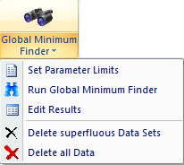
which should be applied in the following way:
1.Import the Experimental CV
In the first step the experimental current curves have to be imported into the Tab-Window: Experiments and all required info (not contained in the ASCII-files) has to be added to each CV as described above or shown in a video clip.
2.Selecting Parameters for being optimized
The selection of parameters which are to be optimized is accomplished as described for the Ribbon Bar Command: Edit. However, when working with the Global Minimum Finder the parameter values entered here do not play the role of starting parameters. They are only used to set default values for the upper and lower limit of the parameter values. If the "real" value is beyond these limits the Global Minimum Finder will not be able to find the optimal parameter set.
3.Defining the Upper and Lower Limit for each Parameter Value 
This command opens a dialog box that enables the user to overwrite the default values for the upper and lower limit associated with each parameter supposed to be optimized. In the case of the CV-example project contained in the file FittingExample.dep the dialog box should look as follows
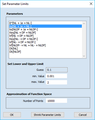
The value shown for Guess cannot be modified. Before the Run command has been executed the value entered in Step 2 is only used to set up the default limits shown in min. Value and max. Value, respectively. If the Global Minimum Finder is iteratively applied, the entry in Guess is the value estimated on the basis of the last finding process (see below). In this case it may be useful to enter new parameter limits or to Shrink Parameter Limits by clicking the button with the same name before restarting the finder.
The value entered in Number of Points indicates how many points (parameter combinations) will be generated in the space spanned by the entirety of parameters taking the upper and lower limits in consideration.
4.Running the Global Minimum Finder 
When running the Global Minimum Finder each parameter combination will be applied to each current curve displayed in the Tab-Window: Experiments. Finally the standard deviation between simulation and experiment will be calculated for the entirety of CVs referring to one and the same parameter combination. At the end the results will be displayed as described below in Edit Results.
5.Edit Results 
Results are displayed in the form of a list sorted by increasing standard deviations
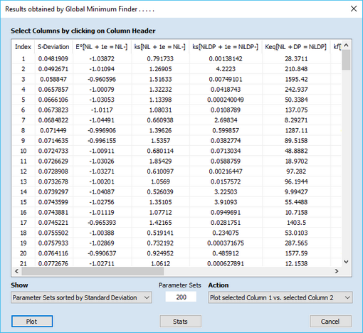
By default 200 Parameter Sets sorted by Standard Deviation are listed when applying the Edit Results command. However, for the most operations provided in Show, Action or Stats the number of Parameter Sets should be restricted to 10-20.
If Show: Parameter Sets sorted by Standard Deviation is selected one of the following actions will be executed when closing the dialog box
oAction: Plot selected Column 1 vs. selected Column 2
This option enables the user to select two columns of data (except those headlined "Index") which are to be plotted in the Tab-Window: Plot Graph after closing the dialog. Usually, the standard deviation is plotted as function of the parameter values to see whether the plot looks like a normal distribution. However, it can also be used to detect parameter correlations.
oAction: Copy selected Parameter Set to Data Fitting
This option enables the user to select a single row of parameter values referring to a particular standard deviation. Note that the caption of the bottom-left button alters from Plot to Copy when choosing this option. After closing the dialog the selected parameter set will be copied to the Data Fitting Project. This enables the user to run either the non-linear fitting procedure (using the copied parameters as starting parameters) or the Global Minimum Finder once more. In the latter case the user is recommended to define new limits for the upper and lower parameter value (closer oriented towards the copied one) before re-running the finder.
oAction: Run Data Fitting for selected Parameter Sets
This option enables the user to select one or more rows of parameter values referring to different standard deviations. Note that the caption of the bottom-left button alters from Plot to Run when choosing this option. After closing the dialog a Data Fitting Project will be created and successively started for each of the selected parameter sets.
If Show: Parameter Correlation has been selected the appearance of the dialog box alters in the following way
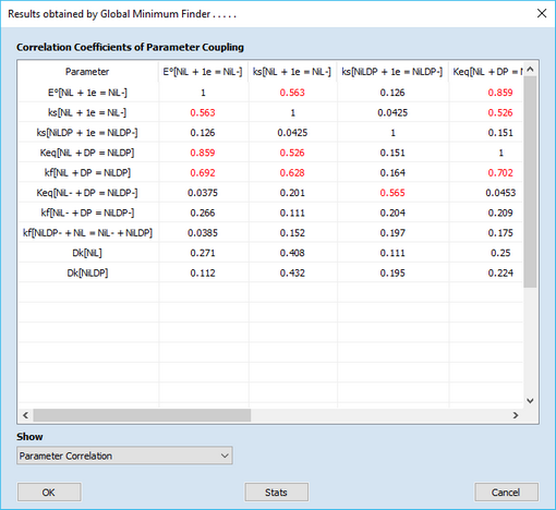
and the correlation coefficients for the individual parameters are displayed in the table. The latter are computed using the parameter values referring to the columns displayed for Show: Parameter Sets sorted by Standard Deviation. For instance, the correlation coefficient between the equilibrium constant of the reaction NiL + DP = NiLDP and the standard potential of NiL + e = NiL
amounts to about 0.86. It has been computed from the values in the columns referring to Keq[NiL + DP = NiLDP] and E°[NiL + e = NiL-] in the higher up dialog restricting the number of Parameter Sets to 15 before switching to Show: Parameter Correlation.
The value is plotted in red because any value larger 0.5 is indicative of a parameter coupling. That means, a modification of Keq can be compensated to some extend by altering E°. Note that "perfect" parameter couplings (which cannot be unraveled mathematically) result usually in correlation coefficients very close to 1. To provide an example the user may think of a reversible charge transfer process followed by a very fast irreversible chemical decomposition reaction. When applying the Global Minimum Finder to a series of CVs representing this mechanism there will be an infinite number of combinations between standard potential and homogeneous rate constant yielding exactly the same standard deviation. Of course, the latter holds true only if an (even larger) infinite number of parameter combinations had been taken into account. In practice the number of Parameter Sets needs to be restricted to a finite but sufficiently large number. In such a situation the Global Minimum Finder may not be able to find the exact value of the global minimum but it will find a certain number of different parameter sets yielding a comparably small standard deviation. When computing the correlation coefficients for such parameter sets a value close to 1 should be retrieved. The proceeding described here will be demonstrated a video clip below.
Button: Stats
Clicking this button opens a dialog box showing minimum, maximum and average parameter value
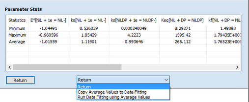
The data refer to the number of Parameter Sets shown/selected when Show: Parameter Sets sorted by Standard Deviation is activated. Three different actions can be executed when closing the dialog.
oAction: Return
The Stats dialog is closed and the program returns to the last status of the Edit Results dialog.
oAction: Copy Average Values to Data Fitting
Note that the caption of the bottom-left button alters from Return to Copy when choosing this option. After closing the dialog the average values are copied to the Data Fitting Project and the Edit Results dialog will be closed, too. This enables the user to run either the non-linear fitting procedure (using the average parameters as starting parameters) or the Global Minimum Finder once more. The parameter values referring to the displayed Minimum and Maximum will be taken as lower and upper limit for the parameter value. However, this choice can be overwritten by the user before re-running the finder.
oAction: Run Data Fitting using Average Values
Note that the caption of the bottom-left button alters from Return to Run when choosing this option. After closing this dialog the average values will be copied to the Data Fitting Project, the Edit Results dialog will be closed, too, and the fitting procedure will be started.
Delete superfluous Data Sets 
Deletes all data sets except those explicitly shown in the higher up dialog. The number of these parameter sets corresponds to the value entered for Parameter Sets. This command should be executed to get rid of a huge amount of superfluous data sets i.e. those resulting in unacceptable large standard deviations. Otherwise all this data will be hold in memory and even stored on hard disk when saving the DigiElch project.
Delete superfluous Data Sets 
Deletes all data sets and resets the upper and lower parameter limit to its default values.
Summary: Play Video
Using the Global Minimum Finder to detect parameter couplings and superfluous reactions
•A series of CVs simulated for a reversible charge transfer process accompanied by a fast irreversible follow-up reaction is used to mimic experimental target curves (ErevCirrev- mechanism). For this purpose, the scan rate used in these simulations varies from 1 to 30 V/s and a constant (relative) level of noise was added to each CV.
•If the follow-up reaction is very there is a (well-known) perfect coupling between the standard potential of the CT-reaction and the rate constant of the homogeneous reaction that cannot be unraveled mathematically. Consequently, subjecting CVs for this kind of mechanism to Data Fitting could lead to unpredictable results if the parameter coupling is not recognized
•In the presented example the analysis of the "experimental" CVs is studied on the basis of a mechanism comprising not only the both reactions actually involved in the ErevCirrev - mechanism but also another follow-up reaction which has no effect on the simulated current curve. This is done to demonstrate the difference between a "superfluous" reaction and a reaction which is absolutely necessary to make the fit working at all even if the "correct" thermodynamic and/or kinetic parameters cannot be determined in some kind of way.
| During the download of the video clip the scrolling of this page may be disabled! |
