DigiElch8 Help

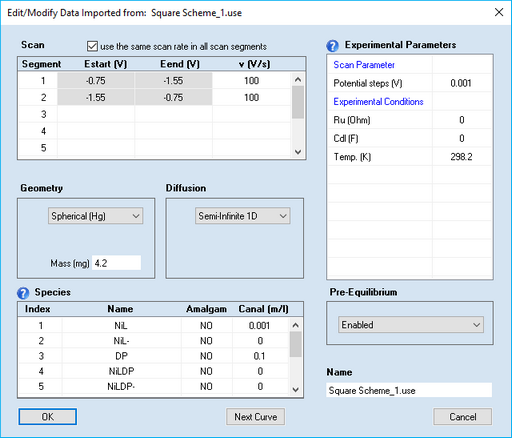
This command opens a dialog box that enables the user to view (or modify) the parameters imported from an experimental data file.

If the Tab-Window: Experiments is empty the active simulation (in the Tab-Window: Simulations)  is used as an template for creating a new experiment before starting the import of the data stored in the ASCII-file. Consequently, if the ASCII-file does only contain voltage/current couples, the parameters associated with the experiment (such as parameters referring to Scan, Pre-Equilibrium, Diffusion, Geometry or Experimental Parameters) will be those of the active simulation. Otherwise (i.e. if the Tab-Window: Experiments is not empty) the active experiment will be taken as the template. If the ASCII-file contains additional information (concerning Scan, Pre-Equilibrium, Diffusion, Geometry or Experimental Parameters) the parameters from the template will be overwritten by the imported ones.

 

 

 

Disabled entries refer to data extracted from the imported curve which should not be modified by the user.

 

1. Scan Parameters:

•Scan segment, v (V/s)
Starting potential, Estart (V), and end-potential, Eend (V), are extracted from the imported current-voltage couples and cannot be modified. The parameter, v (V/s), is the scan rate which can be modified (see below in Scenario 1)

•Check Box: use the same scan rate in each scan segment
Having the option of defining an individual scan rate for each scan segment could lead to more inconvenience for a "classical" CV if the same number had to be entered for each scan segment.  Ticking the check-box use the same value of v(V/s) in each scan segment makes that any modification of the scan rate in one scan segment will be taken over by all other scan segments.

•Check Box: apply background correction
This check-box is visible only if both Ru (Ohm) and Cd (F) are different from zero. Click here for more details.

•Potential steps (V):
The value is extracted from the imported current-voltage couples. If a larger value is entered, the imported current curve is replaced by a cubic-spline interpolation referring to the entered value of Potential steps (V). The dilution of data might be useful for saving computation time when using such files in a fitting project.  

 

2. Pre-Equilibrium

•Disabled
When using the experimental file in a Data Fitting Project the simulation referring to this file will be started using the analytical concentrations, i.e. Cinit = Canal for each species.

•Enabled
When using the experimental file in a Data Fitting Project the equilibrium concentrations of the species will be computed from the analytical concentrations on the basis of the equilibrium constants (chemical and electrochemical ones) entered for the underlying reaction equations. The simulation is started using the equilibrium concentrations as initial concentration, Cinit. This option may lead to unexpected results because the quiet time applied in a "real experiment" is usually not large enough to accomplish that the equilibrium distribution predicted by the Nernst-Equation is obtained in the entire diffusion layer.

•Smart
When using the experimental file in a Data Fitting Project the relation between Estart (V) and the standard potentials, Eo (V), decides whether the analytical concentrations are assigned to the oxidized or reduced form of a redox couple. The initial concentrations are computed then in a second step taking only the chemical reactions into consideration. This option is optimal for all practical purposes unless the user is going to simulate a CV using a starting potential, Estart (V), not quite different from the standard potential, Eo (V).

 

3. Diffusion

•Semi-Infinite 1D
When using the experimental file in a Data Fitting Project the diffusion will be treated in one space direction either by making use of symmetry properties of the electrode or by neglecting contributions from other space directions. The user should be aware that this approach may lead to a considerable error in the current density when approximating a "small" planar (in fact two-dimensional) electrode in terms of an infinitely large (in fact one-dimensional) electrode.

•Finite 1D
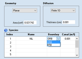
When using the experimental file in a Data Fitting Project the simulation referring to this file is executed for a thin layer electrode. When selecting this mode, a dialog field appears that enables the user to enter the Thickness of the thin layer electrode and the right-hand boundary condition can be selected for each species listed in Species.
 

 

•Semi-Infinite 2D
When using the experimental file in a Data Fitting Project diffusion is simulated in two space directions. This option is much more time consuming because diffusion occurring parallel to the electrode surface is not neglected when using this option.

•Hydrodynamic
diffusion is simulated for a Rotating Disc Electrode (RDE).  When selecting this option, two dialog fields appear which enable the user to enter the rate of rotation, W(rad/s), and the kinematic viscosity, V(cm²/s).

 

4. Geometry

Depending on the selected option for Diffusion the following geometry options are available
 

 

When selecting Spherical (Hg) the user has the choice to specify whether a particular species is going to form an amalgam (i.e. diffusing into the mercury drop) or not. When using the experimental file in a Data Fitting Project the simulation referring to this file will be executed for the specified Geometry.

 

 

5. Experimental Parameters

•Ru (Ohm), Cdl (F)
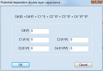
Uncompensated ohmic resistance of the solvent and double layer capacity of the electrode which are to be included into the simulation. Cdl (F) is assumed to have a constant value independently of the potential - a simplification  which does hardly apply to a real electrochemical measurements. Hence, when fitting experimental data the effect of both parameters should be preferably eliminated by using IR-compensation and subtracting the background currents. If the dependence of Cdl (F) on the electrode potential is known and expressible by a polynomial the coefficient of the polynomial approximation can be entered in a dialog box that comes up when clicking with the right mouse button while the cursor is localized over the input field of Cdl (F) :
 

 
Cdl (F) is the constant value of the double layer capacity left over in the limiting case where the dependence of the double layer capacity on the electrode potential expressed by C1, C2, C3 and C4 remains negligibly small. After closing this dialog box only the value of Cdl (F) is displayed in the list of Simulation Parameters but the value of Cdl (F) is written in magenta if one of the coefficients C1, C2, C3, C4 is different from zero.

 

•Temp (K)
The temperature entered in this field is exclusively used for computing the effect of the Nernst-factor. Since DigiElch has no special knowledge about the temperature dependence of thermodynamic and kinetic parameters involved in a particular reaction scheme, it should be obvious, that such information cannot be obtained by executing a series of simulations referring to different temperatures !
 

6. Species

When using experimental files referring to different species concentrations in a Data Fitting Project the user has to add the Name and the analytical concentration, Canal (mol/l), of these species to each experimental file. If the experimental data file does not contain species info, click on the input field headlined Name in the first empty line to enter the name of a new species.  Next to that, the following species parameters can be specified:

 

•Canal (mol/l)
Canal denotes the analytical concentrations of the individual species in mol/l. In the presence of chemical reactions, the analytical concentrations may be different from the equilibrium values, Cinit, (the initial concentrations from which the simulation is actually started). See also "2. Pre-Equilibrium" above.

•Boundary         (only in the case of finite diffusion)
The type of the right-hand boundary can be specified in the associated input fields.

oBRB
"blocked right boundary", i.e. no concentration gradient at the right-hand boundary

oORB
"open right boundary", i.e. concentration values at the right-hand boundary remain constantly at Cinit in the course of the simulation.

•Amalgam        (only if geometry is Spherical (Hg) )
Specify whether a particular species is forming an amalgam (i.e. diffusing into the mercury drop) or not.

 

Why do I need to modify imported data?

The option for modifying experimental parameters may be useful (or even necessary) for the following reasons:

 

Scenario 1: Modifying experimental data imported from ASCII-files which are not compatible with DigiElch's use-file format

ASCII-files (generated by third-party electrochemical hardware) which are not compatible with DigiElch's use-file format do usually not store all relevant experimental conditions in the ASCII file. In many cases, only the experimentally measured CV is stored in the form of voltage-current couples. If the user wants to use such files in a data fitting project, DigiElch needs to know to which experimental parameters (scan rate, electrode size and geometry, diffusion modus, IR-drop, analytical species concentrations etc.) each individual experimental CV refers. This can be done by applying the Edit/Modify command and entering the correct parameters for each imported curve in the dialog box shown on the top of this page. In many cases, there is only one parameter (such as the scan rate) that varies from experiment to experiment while other parameters (such as electrode size and geometry or species concentrations) are constant but not stored in the ASCII-file. In order to avoid that non-varying parameters need to be repeatedly entered for a great number of imported files, the following rules apply:

 

a.If the Tab-Window: Experiments is empty the active simulation (in the Tab-Window: Simulations)  is used as an template for creating a new experiment before starting the import of the data stored in the ASCII-file. Consequently, if the ASCII-file does only contain voltage/current couples, the parameters associated with the experiment (such as parameters referring to Scan, Pre-Equilibrium, Diffusion, Geometry or Experimental Parameters) will be those of the active simulation.
 

b.If the Tab-Window: Experiments is not empty) the active experiment will be taken as the template.
 

c.If the ASCII-file contains additional information (concerning Scan, Pre-Equilibrium, Diffusion, Geometry or Experimental Parameters) the parameters from the template will be overwritten by the imported ones.

 
Scenario 2: Modifying experimental data imported from use-files

The DigiElch use-file format contains a full description of the parameters (such as scan rate, electrode size and geometry, diffusion modus, IR-drop, analytical species concentrations etc.) to which the experiment refers. In other words, if all parameters have been correctly exported to the use-file, any modification after re-importing the file will result in a falsification. Nevertheless, such a falsification may be useful, for instance, for studying how parameter errors (such as a neglected IR-drop or the neglected edge effect resulting from approximating a two-dimensional electrode in terms of a planar one)  is passed to diffusion coefficients and/or  heterogeneous rate constants.