DigiElch8 Help

This command opens a dialog box that enables the user to specify the following parameters referring to the active experiment:

 

 

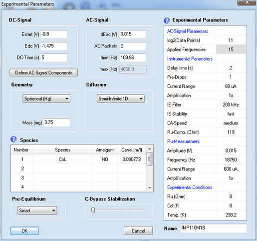
1. DC - Signal

•Estart (V), Edc (V), DC-Time (s)
The experiment is executed in the following way: at the beginning of the experiment the potential of the electrode is assumed to be at Estart (V). Then the electrode potential jumps to Edc (V) and remains at this value for the time indicated by DC-Time (s) before the AC-Signal is superimposed.

2. AC-Signal Parameters

•log2(Data Points)
The number of data points used for generating the AC-signal. It must be an integer power of 2 and is 2^11 = 2048 by default.

•Applied Frequencies
Number of  frequency components from which the multi-sine AC-signal is generated.
 

3. AC - Signal

•dEac (V), AC-Packets, fmin (Hz), fmax (Hz)
The AC-Signal is composed of up to 15 frequencies components which can be edited/defined by clicking on the button Define AC-Signal Components
 

 

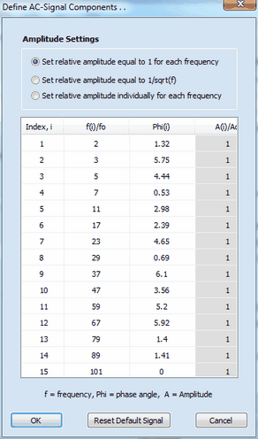
   Each component of the AC-signal is defined by frequency, fi,  phase angle, φi, and amplitude, Ai. These values are relative values referring to the basic frequency, fo  (i.e. the frequency which would be obtained if the signal formed by the 2n data points (where n is the number defined in log2(Data Points)) covers exactly a single sinus cycle.) The overall AC-Signal is generated using the number of frequency components defined in Applied Frequencies. Then the amplitude of the overall signal is adjusted such as to mach the value defined in dEac (V) and the time regime of the simulation is adjusted in such a way that the lowest frequency component is equal to fmin (Hz). The "real world" value of the  highest frequency component, fmax (Hz), depends on the number of Applied Frequencies and the value entered for fmin (Hz). The overall AC-Signal is repeatedly applied n-times where n is the number defined in AC-Packets. Consequently, AC-Packets = 2 means that the overall signal is applied twice in the course of the simulation while the Fourier-Transformation is always executed for the last of the applied AC-Packets.
A simulation referring to an IMP-experiment starts with computing the concentration referring to Estart (V) and the selected Pre-Equilibrium  condition. In the next step the concentration profiles referring to the potential Edc (V) at the end of DC-Time are simulated. Then the simulation of the concentration profiles is continued taking also the superimposed AC-Signal into consideration. At the end of the simulation the current simulated for the last AC-Packet and the applied electrode potential are analyzed by Fourier transformation. In the last step, the real and imaginary part of the impedance is computed from these data for each frequency component.

4. Pre-Equilibrium

•Disabled , Enabled, Smart
When using the IMP-experiment in a Data Fitting Project the simulation(s) will be forced to be executed for the selected Pre-Equilibrium option.

5. Diffusion

•Semi-Infinite 1D
When using the experimental file in a Data Fitting Project the diffusion will be treated in one space direction either by making use of symmetry properties of the electrode or by neglecting contributions from other space directions. The user should be aware that this approach may lead to a considerable error in the current density when approximating a "small" planar (in fact two-dimensional) electrode in terms of an infinitely large (in fact one-dimensional) electrode.

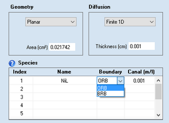
•Finite 1D
When using the experimental file in a Data Fitting Project the simulation referring to this file is executed for a thin layer electrode. When selecting this mode, a dialog field appears that enables the user to enter the Thickness of the thin layer electrode and the right-hand boundary condition can be selected for each species listed in Species.
 

 

•Semi-Infinite 2D
When using the experimental file in a Data Fitting Project diffusion is simulated in two space directions. This option is much more time consuming because diffusion occurring parallel to the electrode surface is not neglected when using this option.

•Hydrodynamic
diffusion is simulated for a Rotating Disc Electrode (RDE).  When selecting this option, two dialog fields appear which enable the user to enter the rate of rotation, W(rad/s), and the kinematic viscosity, V(cm²/s).

When using the experimental CV in a Data Fitting Project the simulation(s) will be forced to be executed for the selected mode of Diffusion and Boundary condition.

 

6. Geometry

Depending on the selected option for Diffusion the following geometry options are available
 

 

When selecting Spherical (Hg) the user has the choice to specify whether a particular species is going to form an amalgam (i.e. diffusing into the mercury drop) or not (see point 8).

 
When using the experimental file in a Data Fitting Project the simulation referring to this file will be executed for the specified Geometry.

 

 

7. Experimental Parameters

Instrumental Parameters

•Delay time (s)
The time elapsing before starting the experiment. When working with an automated mercury drop electrode a delay time of a few second is required to minimize the convection effected by the growth of the mercury drop.
 

•Pre-Drops
When working with an automated mercury drop electrode n+1 mercury drops are produced (where n is the number of Pre-Drops) but the experiment is executed only at the last drop. Helps to improve the reproducibility of the produced mercury drops.
 

•Current Range
The Current Range of the potentiostat used in the experiment. (see Potentiostat's manual for more details)
 

•Amplification
The factor with which the originally measured current signal is amplified by the potentiostats hardware. (see  Potentiostat's manual for more details)
 

•IE-Filter
Setting of the hardware filter applied to the originally measured current signal. (see  Potentiostat's manual for more details)
 

•IE-Stability
The stability setting (applied to the current-to-voltage-converter) of the potentiostat (see  Potentiostat's manual for more details)
 

•CA-Speed
The speed setting of the control-amplifier in the potentiostat (see  Potentiostat's manual for more details)
 

•Ru-Compensation (Ohm)
Value of the ohmic resistance that will be compensated for by positive feedback (from the output of the current-to-voltage-converter to the input of the control-amplifier).

 

Ru-Measurement

•Amplitude (V)
Amplitude of the AC-Signal used for measuring the uncompensated ohmic resistance, Ru (Ohm), and the double layer capacity, Cdl (F).
 

•Frequency (Hz)
Frequency of the AC-Signal used for measuring the uncompensated ohmic resistance, Ru (Ohm), and the double layer capacity, Cdl (F).
 

•Current Range
The Current Range of the potentiostat with which the measurement of the uncompensated ohmic resistance, Ru (Ohm), and the double layer capacity, Cdl (F) is started. Will be automatically optimized.

 

•Amplification
The post amplification factor used for measuring the uncompensated ohmic resistance, Ru (Ohm), and the double layer capacity, Cdl (F).

 

Experimental Conditions

•Ru (Ohm)
Uncompensated ohmic resistance which has been measured or entered. When using the experimental CV in a Data Fitting Project the simulation(s) will be forced to be executed for an uncompensated ohmic resistance equal to Ru (Ohm) - Ru-Compensation (Ohm).
 

•Cdl (F)
The double layer capacity which has been measured or entered. If the dependence of Cdl (F) on the electrode potential is already known when doing the experiment and expressible in polynomial form it can be entered by clicking with the right mouse button while the cursor is localized over the input field of Cdl (F) :
 

 
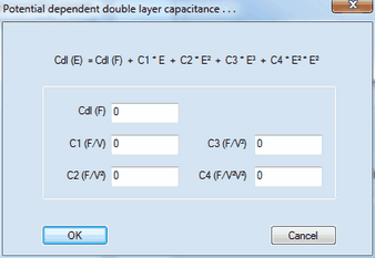
Cdl (F) is the constant value of the double layer capacity left over in the limiting case where the dependence of the double layer capacity on the electrode potential expressed by C1, C2, C3 and C4 remains negligibly small. After closing this dialog box only the value of Cdl (F) is displayed in the list of Experimental Conditions but the value of Cdl (F) is written in magenta if one of the coefficients C1, C2, C3, C4 is different from zero. When using the experimental CV in a Data Fitting Project the simulation(s) will be forced to be executed for these values.
 

•Temp (K)
When using the experimental CV in a Data Fitting Project the simulation(s) will be forced to calculate the Nernst-factor for this temperature.
 

The values entered for Ru (Ohm) and Cdl (F) will be overwritten each time when executing the Command: Measure IR-Drop & Run or IR-Drop.
 

 

8. Species

Click on the first empty input field headlined Species to add a name for each species for which the analytical concentration is explicitly known when running the experiment(s). When using the experimental CV in a Data Fitting Project the simulation(s) will be forced to use the entered analytical concentration provided a species with exactly the same name is found in the mechanism entered for the Data Fitting Project.
 

Entering species concentrations when mixing different volumes of stock solutions
 

1.Enter the names of the underlying species

 

 

 

 

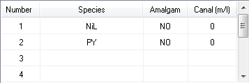
2.Click with the right mouse button on the list containing the species names and enter the volumes and concentrations of the stock solutions from which the sample is prepared.
 

 

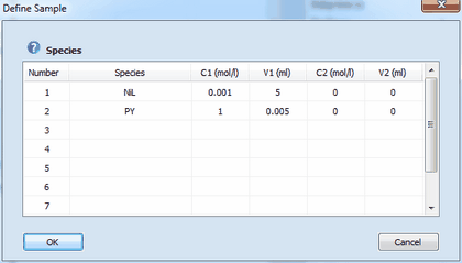
3.The concentration referring to this mixture will be displayed in the Species list after closing the dialog box with OK.

 

9. C-Bypass Stabilization

The stabilization level adjusted at this slider bar takes effect only if the reference and counter electrode are connected by a switchable capacitor shown as shown in the following picture (referring to the Reference 600 Misc I/O Connector)

 

 

 

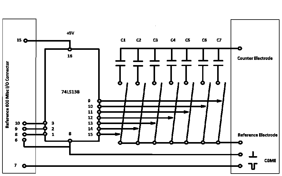
The following capacitors can be recommended:
 

•C1 ≈ 0.1 nF

•C2 ≈ 0.22 nF

•C3 ≈ 0.44 nF

•C4 ≈ 1 nF

•C5 ≈ 2.2 nF

•C6 ≈ 4.7nF

•C7 ≈ 10 nF

 

The optimal value is found by "trial and error". It enables the user to conduct fully IR-compensated CV experiments using scan rates higher than 100 V/s in combination with the CA-Speed level "very fast".

 
Line 7 of the Reference 600 Misc I/O Connector can be used to trigger the generation of a mercury drop for a Controlled Growth Mercury Electrode (see, for instance, the CGME distributed by BASi).